오늘은 CNN의 기초 개념들에 대해 공부해볼 생각이다. 지금까지의 개념들을 수학적인 개념들을 이해하게 되면, 알고리즘 역시 이해가 가는 수준이었는데, 여기서부터는 개발하고 정의한 사람들의 아이디어를 이해하고, 그 아이디어로 실제 구현해가는 과정을 이해하는 게 좀 더 중요해진 것 같다. 오늘도 막무가내로 일단 들이받아보자.
목차
1. 이미지 분석에서의 뉴런 네트워크, 다층 퍼셉트론의 문제점
1.1 픽셀의 RGB 값들로 고양이인지 아닌지 알 수 있어?
- 이미지 크기가 더 커진다면?
- 고양이인지 아닌지를 픽셀의 RGB로 분류할 수 없음
2. Convolutional Layer
2.1 3x3 window, blurring, sharpening
2.1.1 흑백 이미지 만들기
2.1.2 NxN window, blur처리
2.1.3 NxN filter, 부드러운 blur처리
2.1.4 다양한 모양의 filter
2.1.5 정규분포의 확률 밀도 함수를 이용한 filter
2.2 복수의 filter
2.3 복수의 input
2.4 복수의 input과 복수의 filter, conv2d
3. Conv2D Layer Class화
3.1 Input data -> Layer 1 과정
3.2 Input data -> Layer 1 -> Layer 2
3.3 Make Layer Class
3.4 Make Model Class
4. Convolutional Layer for loop remove
4.1 for loop의 비효율
4.2 for loop의 동작 과정 with index
4.3 for loop의 동작 과정 with window
4.4 Vectorization(벡터화)
1. 이미지 분석에서의 뉴런 네트워크, 다층 퍼셉트론의 문제점
앞선 미니 프로젝트의 주제들은 컴퓨터가 "정량"적인 데이터를 분석해 "정량"적인 결과를 내놓았다. 거리, RGB의 값 등 input에 대응되는 같은 차원의 output을 도출해내면 되는 문제들이었다. 그런데 이미지 분석은 조금 다른 차원의 고민을 하게 한다.
1.1 픽셀의 RGB 값들로 고양이인지 아닌지 알 수 있어?

컴퓨터가 분석하기 위해 이 고양이 사진을 (height, width, 3(RGB))의 데이터로 만들자.
그리고 데이터를 input으로 기존 뉴런 레이어를 이용해보자.
당장 생각할 수 있는 방법은 input의 모양을 flatten 시켜 (height * width * 3, )의 shape으로 투입해보자.

이 방법은 두 가지 문제를 일으킨다.
- 이미지 크기가 더 커진다면?
: 고양이 사진의 크기가 30 * 50 정도로 작을 경우는 모르겠지만, 3000 * 5000이라면? 이미지가 수천 장이라면? 데이터의 크기가 조금이라도 커지면, 너무 효율이 떨어지게 된다.
- 고양이인지 아닌지를 픽셀의 RGB로 분류할 수 없음
: 앞선 서술한 것처럼 지금부터 진행해야 하는 분석은 "정량"적인 분석이 아니라는 것이다.
모든 데이터를 flatten 시켜 input으로 투입하는 방식은
같은 고양이더라도 살짝만 고개를 꺾거나 왼쪽, 오른쪽으로 살짝 이동하거나 밤에 찍어 주변이 어두운 상태일 경우 너무나도 다른 RGB 값이 나올 것이다.
이 다양한 범주의 데이터들을 하나의 분류로 본다면, 다른 것들과의 분류가 가능할까? 굉장히 어려운 문제일 것이다.

이 문제들을 어떻게 해결할 수 있을까? 사람들이 사진을 보고 사물을 어떻게 판별하는 걸까? 컴퓨터가 이미지를 이미지 자체로 받아들이도록 하는 방법은 없을까? 이와 같은 질문의 대답을 찾는 과정에서 여러 가지 대안들이 나왔고, 우리는 오늘 그중 하나를 배워볼 것이다.
2. Convolutional Layer
Convolutional Layer를 검색해보면, CNN(Convolutional neural network), 합성곱 신경망이라는 키워드가 나온다. Convolutional Layer는 "합성곱 층"으로 번역되며, CNN의 구성요소로 분류된다.
그 CNN은 "시각적 영상" 분석에 활용되는 인공신경망으로 분류되며, "정규화된 다층 퍼셉트론"으로도 분류된다.
CNN의 주요 구성요소인 Convolutional Layer에 대해 알아보자.
기존 뉴런 네트워크의 flatten data 연산이 가지고 있는 문제점을 보완하고자, Convolutional Layer는 데이터의 "공간적 정보"를 보존해 연산을 진행한다.
여기서의 "공간적 정보"를 보존하는 방법은 matrix 모양의 "window, filter"이다.
2.1 3x3 window, blurring, sharpening
우리는 이제 이미지를 하나의 픽셀로 보는 게 아니라 NxN의 window로 봐볼 것이다.
이 과정을 통해서 "blurring", "sharpening"된 결과물을 얻어볼 것이다.
그리고 이 과정에서 window가 "공간적 정보"를 보존한다는 의미도 이해해보도록 하자.
2.1.1 흑백 이미지 만들기

import numpy as np
import matplotlib.pyplot as plt

img = plt.imread('./고먐미.jpg').astype(np.float32)

print(img.shape)    # (1125, 1125, 3)
우리는 shape (1125, 1125, 3)의 이미지를 분석해 볼 것이다.
일단은 한 픽셀이 RGB 3개로 나눠져 당장은 이해하기 복잡하기에 흑백 이미지로 바꿔보자.

import numpy as np
import matplotlib.pyplot as plt

img = plt.imread('./고먐미.jpg').astype(np.float32)

print(img.shape)    # (1125, 1125, 3)

img_gray = np.mean(img, axis=-1)
print(img_gray.shape)   # (1125, 1125)

fig, ax = plt.subplots(figsize=(20, 20))
ax.imshow(img_gray, cmap="gray")

plt.show()
2.1.2 NxN window, blur처리
이전까지 픽셀 하나하나의 데이터들을 연산했다면, 우리는 이제 NxN window의 데이터들을 연산해 볼 것이다.
먼저 3x3 window로 데이터를 받아 연산한 후 데이터를 쌓아보자
연산하는 과정은 아래 그림과 같다

그럼 실제 구현해보자!
import numpy as np
import matplotlib.pyplot as plt
from numpy.lib.index_tricks import nd_grid

img = plt.imread('./고먐미.jpg').astype(np.float32)

print(img.shape)    # (1125, 1125, 3)

img_gray = np.mean(img, axis=-1)
print(img_gray.shape)   # (1125, 1125)

n_window = 3
H, W = img_gray.shape

h_w =  np.round(H/n_window).astype(np.int32)
w_w = np.round(W/n_window).astype(np.int32)
print(h_w, w_w)

result = np.empty(shape=(h_w,w_w))
for h_idx in range(h_w):
    for w_idx in range(w_w):
        window = img_gray[h_idx*n_window : h_idx*n_window+n_window,
                            w_idx*n_window : w_idx*n_window+n_window]
        mean = np.mean(window)
        result[h_idx, w_idx] = mean

fig, ax = plt.subplots(1, 2, figsize=(20, 20))
ax[0].imshow(img_gray, cmap="gray")
ax[1].imshow(result, cmap="gray")

plt.show()
어? 3x3 window의 데이터의 평균들을 모아서 이미지를 그려봤더니 원본 이미지와 차이가 없다!? 그럴 리가 없는데,
window의 크기를 늘려보자
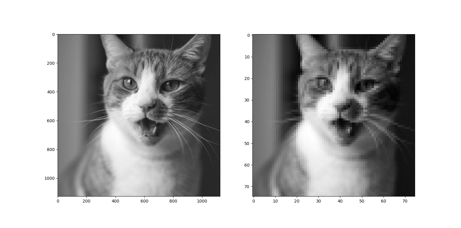
아 15x15 window를 활용했더니 이제야 픽셀들의 각진 구분선들이 보이고, 블러 처리가 된듯한 이미지가 출력된다.
우리는 이 챕터를 통해 이미지 데이터를 matrix형태의 window 단위로 나눠서 연산 및 처리할 수 있게 됐다.
위에서 구현한 window 방식과 비슷한 방식인 filter도 살펴보자
2.1.3 NxN filter, 부드러운 blur처리
filter방식은 NxN window와 비슷하지만, 좀 더 복잡한 연산을 가능하게 하는 구조이다. matrix 모양의 데이터 각각과 연산을 할 수 있게 돕는다.
코드를 통해 살펴볼 예정인데, CNN의 데이터 처리 방법이기도 하여 "중첩"해 filter, window를 뽑는 방식으로 데이터 연산을 진행할 것이다. 위에서 진행했던 방식과 달라 아래 그림으로 설명하겠다.
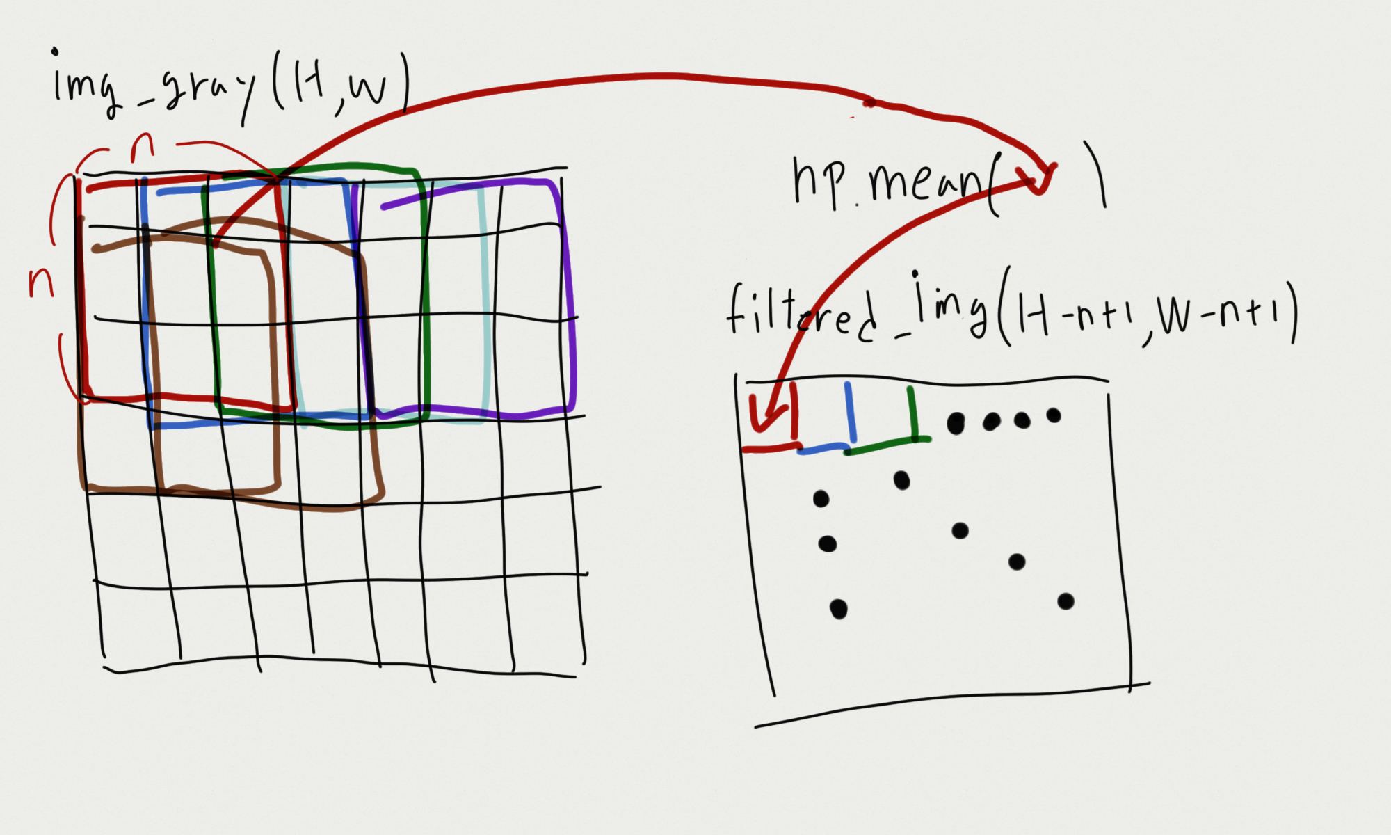
그림과 같이 filter를 중첩하여 연산을 진행할 것이고, 관련해 window, filter의 크기에 따라 for문의 범위를 정하는 공식 역시 코드를 통해 보여주겠다. 위 구현 코드와 비교하며, 살펴보도록 하자.
코드를 통해 중첩 filter 처리를 구현해보겠다.
import numpy as np
import matplotlib.pyplot as plt

img = plt.imread('./고먐미.jpg').astype(np.float32)

# print(img.shape)    # (1125, 1125, 3)

img_gray = np.mean(img, axis=-1)
# print(img_gray.shape)   # (1125, 1125)

H, W = img_gray.shape   # image의 Height, Width

# 15x15 filter
H_F_15, W_F_15 = 15,15  # filter의 Height, Width / 보통 filter는 NxN의 형식으로 Height와 Width를 동일하게 설정함
mean_filter_15 = np.full(fill_value=(1 / (H_F_15 * W_F_15)), shape=(H_F_15, W_F_15))     # (15*15)^-1 = 0.00444... , (15, 15)
n_H_15 = H - H_F_15 + 1
n_W_15 = W - W_F_15 + 1

# filtered image by 15x15 filter
filtered_img_15 = np.empty(shape=(n_H_15, n_W_15))

# 연산
for h_idx in range(n_H_15):
    for w_idx in range(n_W_15):
        window = img_gray[h_idx : h_idx + H_F_15,
                         w_idx : w_idx + W_F_15]
        mean = np.sum(window * mean_filter_15)
        filtered_img_15[h_idx, w_idx] = mean

# 30x30 filter
H_F_30, W_F_30 = 30,30
mean_filter_30 = np.full(fill_value=(1 / (H_F_30 * W_F_30)), shape=(H_F_30, W_F_30))    # (30*30)^-1 (30, 30)
n_H_30 = H - H_F_30 + 1
n_W_30 = W - W_F_30 + 1

# filtered image by 30x30 filter
filtered_img_30 = np.empty(shape=(n_H_30, n_W_30))

# 연산
for h_idx in range(n_H_30):
    for w_idx in range(n_W_30):
        window = img_gray[h_idx : h_idx + H_F_30,
                         w_idx : w_idx + W_F_30]
        mean = np.sum(window * mean_filter_30)
        filtered_img_30[h_idx, w_idx] = mean

fig, ax = plt.subplots(1, 3, figsize=(20, 20))
ax[0].imshow(img_gray, cmap="gray")
ax[1].imshow(filtered_img_15, cmap="gray")
ax[2].imshow(filtered_img_30, cmap="gray")

plt.show()
원본 이미지 h, w가 1000이 넘어가서 그런지 3x3으론 티도 안 나서 30x30으로 바꿔봤다. 아까 중첩을 안 한 상태로 window를 나눠 mean 연산을 했을 때보다 조금 더 부드럽게 블러 처리가 됐다.
내가 이 구현 과정을 통해서 느낀 점이 있다.
window, filter 데이터를 통해 연산하게 되면, 그 데이터들이 이전보다 조금 더 많은 "정보"를 담고 있다는 것을 알게 됐다. 하나의 픽셀일 때는 점에 불과했던 것들이 하나의 선, 경계를 나타내는 데이터가 된다는 것이다.
이 데이터들을 수학적으로 가공하면, 의미 있는 처리가 가능하지 않을까?
2.1.4 다양한 모양의 filter
1.
[1 0 -1] [1 1 1]
[1 0 -1] [0 0 0]
[1 0 -1] [-1 -1 -1]
import numpy as np
import matplotlib.pyplot as plt

# 이미지가 너무 커 size를 줄였습니다
img = plt.imread('./고먐미.jpg').astype(np.float32)
# img = plt.imread('./building.jpg').astype(np.float32)

print(img.shape)    # (500, 500, 3)

img_gray = np.mean(img, axis=-1)
# print(img_gray.shape)   # (500, 500)

H, W = img_gray.shape   # image의 Height, Width
n_F = 3

v_filter = np.array([[1, 0, -1],
                    [1, 0, -1],
                    [1, 0, -1]])
n_H = H - n_F + 1
n_W = W - n_F + 1
v_filtered_img = np.empty(shape=(n_H, n_W))

# 연산
for h_idx in range(n_H):
    for w_idx in range(n_W):
        window = img_gray[h_idx : h_idx + n_F,
                         w_idx : w_idx + n_F]
        z = np.sum(window * v_filter)
        v_filtered_img[h_idx, w_idx] = z

h_filter = np.array([[1, 1, 1],
                    [0, 0, 0],
                    [-1, -1, -1]])
n_H = H - n_F + 1
n_W = W - n_F + 1
h_filtered_img = np.empty(shape=(n_H, n_W))

# 연산
for h_idx in range(n_H):
    for w_idx in range(n_W):
        window = img_gray[h_idx : h_idx + n_F,
                         w_idx : w_idx + n_F]
        z = np.sum(window * h_filter)
        h_filtered_img[h_idx, w_idx] = z

fig, ax = plt.subplots(1, 3, figsize=(20, 20))
ax[0].imshow(img_gray, cmap="gray")
ax[1].imshow(v_filtered_img, cmap="gray")
ax[2].imshow(h_filtered_img, cmap="gray")

plt.show()

2.
import numpy as np
import matplotlib.pyplot as plt

def filtering(img, filter):
    H, W = img.shape
    h_F, w_F = filter.shape
    n_H = H - h_F + 1
    n_W = W - w_F + 1
    filtered_img = np.empty(shape=(n_H, n_W))
    # 연산
    for h_idx in range(n_H):
        for w_idx in range(n_W):
            window = img[h_idx : h_idx + h_F,
                            w_idx : w_idx + w_F]
            z = np.sum(window * filter)
            filtered_img[h_idx, w_idx] = z
    return filtered_img

img = plt.imread('./고먐미.jpg').astype(np.float32)
img_gray = np.mean(img, axis=-1)

fig, ax = plt.subplots(3, 2)

ax[0,0].imshow(img_gray, cmap="gray")
ax[0,1].imshow(img_gray, cmap="gray")

## 1
filter = np.array([[1,-1,-1, 1],
                    [1,-1,-1,1],
                    [1,-1,-1,1],
                    [1,-1,-1, 1]])
ax[1, 0].imshow(filtering(img_gray, filter), cmap="gray")

## 1-1
filter = np.array([[1,0,0,-1],
                    [1,0,0,-1],
                    [1,0,0,-1],
                    [1,0,0,-1]])
ax[1, 1].imshow(filtering(img_gray, filter), cmap="gray")

filter = np.array([[1,1,1,1],
                    [-1,-1,-1,-1],
                    [-1,-1,-1,-1],
                    [1,1,1, 1]])
ax[2, 0].imshow(filtering(img_gray, filter), cmap="gray")

filter = np.array([[1,1,1,1],
                    [0,0,0,0],
                    [0,0,0,0],
                    [-1,-1,-1,-1]])
ax[2, 1].imshow(filtering(img_gray, filter), cmap="gray")

plt.tight_layout()
plt.show()
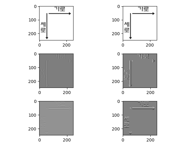

[1 0 -1]에서 0의 의미, 그림으로 생각해보자

자료 찾아보며, 의미 있는 결과를 찾는데 시간이 좀 걸렸다.
위 코드와 같이 가로, 세로 선을 구분할 수 있도록 filter를 설정하면, 위 그림과 같은 결과를 얻을 수 있다.
이 개념을 이용하면, 선 이외에도 곡선과 특정한 모양(고양이의 귀, 사람의 코, 눈동자) 등을 캐치해낼 수 있을 것 같다.
* 도움된 영상
- https://www.youtube.com/watch?v=7PZDbTfvDIQ
2.1.5 정규분포의 확률 밀도 함수를 이용한 filter
수학적 이해가 부족해서... 위 작업과 어떻게 이어지는 게 설명을 못하겠다.
수식, 수식을 이용한 구현과 결과를 나열하는 것으로 챕터를 마무리하겠다.
$$ \frac{1}{\sqrt{2\pi}\sigma} e^{-\frac{(x- \mu)^{2}}{2\sigma^{2}}}\;(-\infty<x<\infty)$$
import numpy as np
import matplotlib.pyplot as plt

def filtering(img, n_F, sigma):

    half_filter_size = (n_F - 1) / 2
	H, W = img.shape   # image의 Height, Width

    x = np.arange(-half_filter_size, half_filter_size + 1)
    y = np.arange(-half_filter_size, half_filter_size + 1)

    X, Y = np.meshgrid(x, y)

    gaussian_constant = 1 / (2 * np.pi * (sigma))
    gaussian_exp = np.exp(-1 * (X ** 2 + Y ** 2) / (2 * (sigma ** 2)))
    filter = gaussian_constant * gaussian_exp

    n_H = H - n_F + 1
    n_W = W - n_F + 1

    filtered_img = np.empty(shape=(n_H, n_W))

    # 연산
    for h_idx in range(n_H):
        for w_idx in range(n_W):
            window = img[h_idx : h_idx + n_F,
                            w_idx : w_idx + n_F]
            z = np.sum(window * filter)
            filtered_img[h_idx, w_idx] = z

    return filtered_img

# 이미지가 너무 커 size를 줄였습니다
img = plt.imread('./고먐미.jpg').astype(np.float32)

print(img.shape)    # (500, 500, 3)

img_gray = np.mean(img, axis=-1)
# print(img_gray.shape)   # (500, 500)

fig, ax = plt.subplots(2, 2, figsize=(20, 20))
ax[0,0].imshow(filtering(img=img_gray, n_F=15, sigma=1), cmap="gray")
ax[0,1].imshow(filtering(img=img_gray, n_F=15, sigma=3), cmap="gray")
ax[1,0].imshow(filtering(img=img_gray, n_F=30, sigma=1), cmap="gray")
ax[1,1].imshow(filtering(img=img_gray, n_F=30, sigma=3), cmap="gray")

plt.show()
filter의 size보다 σ, 표준편차에 더 큰 영향을 받는 걸 알 수 있다.
짧은 수학 상식으로 생각해보면, 표준 편차가 커진다는 것은 정규 분포한 데이터들 간의 거리가 더 멀어진다는 것을 의미하기에 더 흐려질 것이다.
2.2 복수의 filter
위 챕터에서 CNN과 연결해 이야기해보자면,
하나의 이미지 데이터에 복수 필터를 이용해 복수의 결괏값을 얻었다.
같은 데이터를 두고도 여러 분석, 결과물을 도출하는 것이다.

import numpy as np
import matplotlib.pyplot as plt

img = plt.imread('고먐미.jpg')
img_ = img.astype(np.float32)
img_gray = np.mean(img_, axis=-1)

filters = list()
filter1 = np.array([[1,1,1,1,1],
                    [0,0,0,0,0],
                    [0,0,0,0,0],
                    [0,0,0,0,0],
                    [-1,-1,-1,-1,-1]])
filter2 = np.array([[1,0,0,0,-1],
                    [1,0,0,0,-1],
                    [1,0,0,0,-1],
                    [1,0,0,0,-1],
                    [1,0,0,0,-1]])
filter3 = np.full(fill_value=1/(15*15), shape=(15, 15))
filter4 = np.full(fill_value=1/(30*30), shape=(30, 30))

filters.append(filter1)
filters.append(filter2)
filters.append(filter3)
filters.append(filter4)

H, W = img_gray.shape

filtered_img_list = list()
for f_idx in range(len(filters)):
    filter = filters[f_idx]
    n_F = filter.shape[0]
    H_F, W_F = H - n_F + 1, W - n_F + 1
    filtered_img = np.empty(shape=(H_F, W_F))
    for h_idx in range(H_F):
        for w_idx in range(W_F):
            window = img_gray[h_idx : h_idx + n_F,
                            w_idx : w_idx + n_F,]
            z = np.sum(window * filter)
            filtered_img[h_idx, w_idx] = z

    filtered_img_list.append(filtered_img)

fig, ax = plt.subplots(1,(len(filtered_img_list)+1), figsize=(10, 10))
ax[0].imshow(img)

for f_idx in range(len(filtered_img_list)):
    filtered_img = filtered_img_list[f_idx]
    ax[f_idx+1].imshow(filtered_img, cmap="gray")

plt.show()

하나의 데이터를 다양한 filter로 다양한 결과물을 도출할 수 있다면,
각각의 filter들을 각각 특정 "모양, 선" 등을 필터링하는 역할을 하게 하고,
뉴런 네트워크와 같은 방식을 활용해서
"특정 모양, 선"을 포함 = "특정한 사물"로 분류하는 방식도 가능하지 않을까?
우리가 배웠던 뉴런 네트워크는
하나의 레이어에 복수의 뉴런이 있고, 그 뉴런이 각각 w(가중치)를 가지고, 레이어의 b(상수)를
가지는 식으로 구성돼있다.
이 방식을 차용해 "filter의 요소"들을 "특정 모양을 구분하는 가중치 혹은 상수"로 바라볼 수도 있지 않을까?
이미지 분석을 뉴런 네트워크화하기 위해 먼저 input을 복수로 만들어보자
2.3 복수의 input
그림으로 보자면

코드로 보자면
import numpy as np
import matplotlib.pyplot as plt

img = plt.imread('고먐미.jpg')
img_ = img.astype(np.float32)

def filtering(img, n_F, n_C_out):
    H, W, n_C_in = img.shape   # Height, Width, 입력 채널 수

    filter = np.full(fill_value=(1/(n_F * n_F)), shape=(n_F,n_F))
    H_F, W_F = H - n_F + 1, W - n_F + 1
    filtered_img = np.empty(shape=(H_F, W_F, n_C_out))

    for c_idx in range(n_C_out):
        for h_idx in range(H_F):
            for w_idx in range(W_F):
                window = img_[h_idx: h_idx+n_F,
                            w_idx: w_idx+n_F, c_idx]
                z = np.sum(window * filter)
                filtered_img[h_idx, w_idx, c_idx] = z

    filtered_img = filtered_img.astype(np.int32)

    return filtered_img

fig, ax = plt.subplots(1,3,figsize=(20, 20))
ax[0].imshow(img)
ax[1].imshow(filtering(img=img_, n_F=15, n_C_out=3))
ax[2].imshow(filtering(img=img_, n_F=30, n_C_out=3))

plt.show()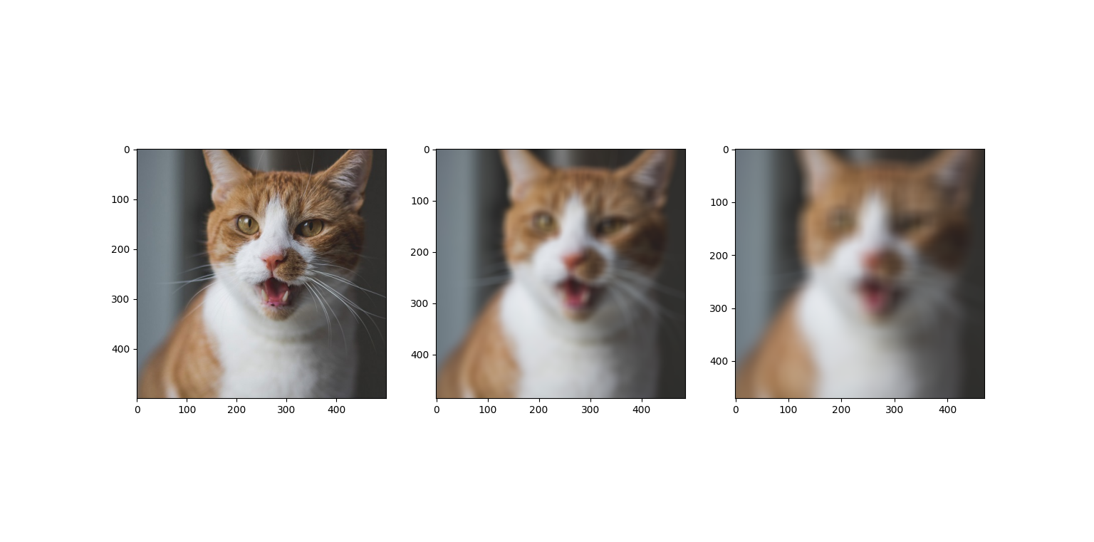
RGB 값을 3개의 input으로 만들어 하나의 filter를 3번 통과해 값을 쌓아봤다.
그러니, 컬러인 상태에서 blur처리가 된 모습을 볼 수 있었다.
그러면 복수 input가 복수 filter를 각각 통과해보면 어떨까?
2.4 복수의 input과 복수의 filter, conv2d
그림으로 보자면

코드로 보자면
import numpy as np
import matplotlib.pyplot as plt

img = plt.imread('고먐미.jpg')
img_ = img.astype(np.float32)

H, W, n_C_in = img.shape   # Height, Width, 입력 채널 수

filters = list()
filter1 = np.array([[1,1,1,1,1],
                    [0,0,0,0,0],
                    [0,0,0,0,0],
                    [0,0,0,0,0],
                    [-1,-1,-1,-1,-1]])
filter2 = np.array([[1,0,0,0,-1],
                    [1,0,0,0,-1],
                    [1,0,0,0,-1],
                    [1,0,0,0,-1],
                    [1,0,0,0,-1]])
filter3 = np.full(fill_value=1/(15*15), shape=(15, 15))
filter4 = np.full(fill_value=1/(30*30), shape=(30, 30))

filters.append(filter1)
filters.append(filter2)
filters.append(filter3)
filters.append(filter4)

filtered_img_list = list()

for f_idx in range(len(filters)):
    filter = filters[f_idx]
    n_F = filter.shape[0]
    H_F, W_F = H - n_F + 1, W - n_F + 1
    filtered_img = np.empty(shape=(H_F, W_F, n_C_in))
    for c_idx in range(n_C_in):
        img_single = img_[...,c_idx]
        for h_idx in range(H_F):
            for w_idx in range(W_F):
                window = img_single[h_idx : h_idx + n_F,
                                    w_idx : w_idx + n_F]
                z = np.sum(window * filter)
                filtered_img[h_idx, w_idx, c_idx] = z

    filtered_img_list.append(filtered_img)

print(len(filtered_img_list))

fig, ax = plt.subplots(1, (len(filtered_img_list)+1), figsize=(10, 20))
ax[0].imshow(img)

for i in range(len(filtered_img_list)):
    filtered_img = filtered_img_list[i]
    filtered_img = filtered_img.astype(np.int32)
    ax[i+1].imshow(filtered_img, cmap="gray")

plt.show()
복수의 input을 RGB 각각의 값으로 투입했기에, 컬러 이미지로 쌓을 수 있었다.
이 개념을 좀 더 추상화해서 살펴보자. 이미지 (H, W, 3(RGB)) 기준의 input 말고! 더 많은 filter로!
import numpy as np
from numpy.random import normal

H_in, W_in, C_in = 200, 300, 3  # input data의 Height, Width, Channel의 개수
F, C_out = 5, 20                # output Filter의 크기, output Channel의 개수

X = normal(0, 1, (H_in, W_in, C_in))    # input data X / (Height, Width, Channel의 개수)
filter_ = normal(0, 1, (F, F, C_in, C_out)) # 하나의 layer의 filter들, input Channel에 따라서도 다른 filter
# W = normal(0, 1, (F, F, C_in, C_out)) # 하나의 layer의 filter들(="가중치들")
B = normal(0, 1, (C_out, )) # 하나의 layer의 하나의 output의 상수들

H_out, W_out = H_in - F + 1, W_in - F + 1   # input data에 따른 filter들의 중첩 동작 범위(H_in에 따른, W_in에 따른)

A = np.empty(shape=(H_out, W_out, C_out))   # 필터링된 output

for c_idx in range(C_out):
    c_filter = filter_[..., c_idx]
    c_b = B[c_idx]
    for row_idx in range(H_out):
        for col_idx in range(W_out):
            window = X[row_idx : row_idx + F,
                        col_idx : col_idx + F]
            z = np.sum(window * c_filter) + c_b
            a = 1/(1 + np.exp(-z))

            A[row_idx, col_idx, c_idx] = a

print(A.shape)

# Layer 2 A가 X를 대체
H_in, W_in, C_in = A.shape

"""
... 솰라솰라
"""
이렇게 되면, 뉴런 네트워크의 이미지 데이터 버전이 완성된다.
우리는 이 네트워크를 "conv2d"라고 부른다.

conv2d는 가장 기본적인 convolution layer(합성곱 레이어)로서 이미지 형식의 다차원 데이터를 "공간적 정보"를 유지한 채 연산 및 처리를 할 수 있게 한다.
여기서 filter와 b(bias 상수)의 역할은 추후에 좀 더 깊게 포스팅하겠다.
3. Conv2D Layer Class화
3.1 Input data -> Layer 1 과정
import numpy as np
from numpy.random import normal

H_in, W_in, C_in = 200, 300, 3
F, C_out = 5, 20

# Input Data
X = normal(0, 1, (H_in, W_in, C_in))
print(X.shape)  # (200, 300, 3)

# Layer 1
filter_ = normal(0, 1, (F, F, C_in, C_out)) # 하나의 layer의 filter들, input Channel에 따라서도 다른 filter
B = normal(0, 1, (C_out, )) # 하나의 layer의 하나의 output의 상수들

H_out, W_out = H_in - F + 1, W_in - F + 1

# Layer 1 output
A = np.empty(shape=(H_out, W_out, C_out))

# Layer1 연산
for c_idx in range(C_out):
    c_filter = filter_[..., c_idx]
    c_b = B[c_idx]
    for row_idx in range(H_out):
        for col_idx in range(W_out):
            window = X[row_idx : row_idx + F,
                        col_idx : col_idx + F]
            z = np.sum(window * c_filter) + c_b
            a = 1/(1 + np.exp(-z))

            A[row_idx, col_idx, c_idx] = a

# Layer1 Result
print(A.shape)  # (196, 296, 20)
Input Data : (200, 300, 3)
Layer1 Result : (196, 296, 20)
3.2 Input data -> Layer 1 -> Layer 2
import numpy as np
from numpy.random import normal
import matplotlib.pyplot as plt

H_in, W_in, C_in = 200, 300, 3
F, C_out = 5, 3

# Input Data
X = normal(0, 1, (H_in, W_in, C_in))
print(X.shape)  # (200, 300, 3)

# Layer 1
filter_ = normal(0, 1, (F, F, C_in, C_out)) # 하나의 layer의 filter들, input Channel에 따라서도 다른 filter
B = normal(0, 1, (C_out, )) # 하나의 layer의 하나의 output의 상수들

H_out, W_out = H_in - F + 1, W_in - F + 1

# Layer 1 output
A = np.empty(shape=(H_out, W_out, C_out))

# Layer1 연산
for c_idx in range(C_out):
    c_filter = filter_[..., c_idx]
    c_b = B[c_idx]
    for row_idx in range(H_out):
        for col_idx in range(W_out):
            window = X[row_idx : row_idx + F,
                        col_idx : col_idx + F]
            z = np.sum(window * c_filter) + c_b
            a = 1/(1 + np.exp(-z))

            A[row_idx, col_idx, c_idx] = a

# Layer1 Result
print(A.shape)  # (196, 296, 20)

# Layer2
# Input Data : A
print(A.shape)  # (196, 296, 3)

H_in, W_in, C_in = A.shape
F, C_out = 7, 10

# Layer 2 filter
filter_ = normal(0, 1, (F, F, C_in, C_out))
B = normal(0, 1, (C_out, ))

H_out, W_out = H_in - F + 1, W_in - F + 1

# Layer 2 output
A = np.empty(shape=(H_out, W_out, C_out))

# Layer2 연산
for c_idx in range(C_out):
    c_filter = filter_[..., c_idx]
    c_b = B[c_idx]
    for row_idx in range(H_out):
        for col_idx in range(W_out):
            window = X[row_idx : row_idx + F,
                        col_idx : col_idx + F]
            z = np.sum(window * c_filter) + c_b
            a = 1/(1 + np.exp(-z))

            A[row_idx, col_idx, c_idx] = a

# Layer2 Result
print(A.shape)  # (190, 290, 10)
Input Data : (200, 300, 3)
Layer1 Result : (196, 296, 20)
Lyaer2 Result : (190, 290, 10)
3.3 Make Layer Class
import numpy as np
from numpy.random import normal

class Layer:
    def __init__(self, F, C_out):
        self.F, self.C_out = F, C_out

        self.input = None
        self.H_in, self.W_in, self.C_in = None, None, None

        self.H_out, self.W_out = None, None
        self.filter = None
        self.B = None
        self.A = None

    def _init_params(self, input):
        self.input = input
        self.H_in, self.W_in, self.C_in = input.shape

        self.H_out, self.W_out = self.H_in - self.F + 1, self.W_in - self.F + 1
        self.filter = normal(0, 1, (self.F, self.F, self.C_in, self.C_out))
        self.B = normal(0, 1, (self.C_out, ))
        self.A = np.empty(shape=(self.H_out, self.W_out, self.C_out))

    def __call__(self, input):
        self._init_params(input)

        for c_idx in range(self.C_out):
            c_filter = self.filter[..., c_idx]
            c_b = self.B[c_idx]
            for row_idx in range(self.H_out):
                for col_idx in range(self.W_out):
                    window = self.input[row_idx : row_idx + self.F,
                                col_idx : col_idx + self.F]
                    z = np.sum(window * c_filter) + c_b
                    a = 1/(1 + np.exp(-z))

                    self.A[row_idx, col_idx, c_idx] = a

        return self.A

H, W, C_in = 300, 200, 3
X = normal(0, 1, (H, W, C_in))

layer1 = Layer(F=5, C_out=10)
layer2 = Layer(F=10, C_out=7)
layer3 = Layer(F=15, C_out=3)

print(X.shape)  # (300, 200, 3)

A1 = layer1(input=X)
print(A1.shape) # (296, 196, 10)

A2 = layer2(input=A1)
print(A2.shape) # (286, 187, 7)

A3 = layer3(input=A2)
print(A3.shape) # (273, 173, 3)
Input Data(X) : (300, 200, 3)
Layer1 Result : (296, 196, 10)
Layer2 Result : (286, 187, 7)
Layer3 Result : (273, 173, 3)
3.4 Make Model Class
import numpy as np
from numpy.random import normal

class Model:

    def __init__(self, n_layer, F_list, C_out_list):
        self.n_layer = n_layer
        self.F_list = F_list
        self.C_out_list = C_out_list

    def __call__(self, input):
        X = input
        for layer_idx in range(self.n_layer):
            F = self.F_list[layer_idx]
            C_out = self.C_out_list[layer_idx]
            layer = Layer(F=F, C_out=C_out)
            A = layer(X)
            print(f"Layer{layer_idx+1} result : {A.shape}")
            X = A

        return X

class Layer:
    def __init__(self, F, C_out):
        self.F, self.C_out = F, C_out

        self.input = None
        self.H_in, self.W_in, self.C_in = None, None, None

        self.H_out, self.W_out = None, None
        self.filter = None
        self.B = None
        self.A = None

    def _init_params(self, input):
        self.input = input
        self.H_in, self.W_in, self.C_in = input.shape

        self.H_out, self.W_out = self.H_in - self.F + 1, self.W_in - self.F + 1
        self.filter = normal(0, 1, (self.F, self.F, self.C_in, self.C_out))
        self.B = normal(0, 1, (self.C_out, ))
        self.A = np.empty(shape=(self.H_out, self.W_out, self.C_out))

    def __call__(self, input):
        self._init_params(input)

        for c_idx in range(self.C_out):
            c_filter = self.filter[..., c_idx]
            c_b = self.B[c_idx]
            for row_idx in range(self.H_out):
                for col_idx in range(self.W_out):
                    window = self.input[row_idx : row_idx + self.F,
                                col_idx : col_idx + self.F]
                    z = np.sum(window * c_filter) + c_b
                    a = 1/(1 + np.exp(-z))

                    self.A[row_idx, col_idx, c_idx] = a

        return self.A

H, W, C_in = 300, 200, 3
X = normal(0, 1, (H, W, C_in))

print("input : ", X.shape)

n_layer = 3
F_list = [5, 10, 15]
C_out_list = [10, 7, 3]

model = Model(n_layer=n_layer, F_list=F_list, C_out_list=C_out_list)
result = model(input=X)

print("result : ", result.shape)
Input Data(X) : (300, 200, 3)
Layer1 Result : (296, 196, 10)
Layer2 Result : (287, 187, 7)
Layer3 Result : (273, 173, 3)
Result : (273, 173, 3)
Result가 연산 및 처리된 이미지의 형태인 것을 확인할 수 있다.
4. Convolutional Layer for loop remove
언제나 for문이 문제다. 항상 시간을 잡아먹는 친구다. 그렇지만 numpy 등 데이터 사이언스에서 활용되는 친구들은 내가 활용만 잘하면, for문 없이 빠른 연산을 할 수 있게 돕는다.
여기서 중요한 건 "내가 활용만 잘하면"이다.
4.1 for loop의 비효율
import numpy as np
from numpy.random import randint

H_in, W_in = 1080, 1920

F = 3
X = randint(0, 10, (H_in, W_in))

W = randint(0, 10, (F, F))
B = randint(0, 10, ())
H_out, W_out = H_in - F + 1, W_in - F + 1

print(H_out, W_out) # 1078 1918

Z = np.empty(shape=(H_out, W_out))
for row_idx in range(H_out):
    for col_idx in range(W_out):
        window = X[row_idx : row_idx + F,
                   col_idx : col_idx + F]
        z = np.sum(window * W) + B
        Z[row_idx, col_idx] = z
for문을 이용한 흑백 이미지 한 장을 기준으로 한 convolutional layer 코드이다.
하나의 layer임에도 불구하고 Height: 1080, Width: 1920일 경우
for문은 "H_out * W_out" = "1078 * 1918" = "2,067,604"번 돈다.
시간이 얼마나 걸리는지를 확인해보면
import numpy as np
from numpy.random import randint
from time import time
H_in, W_in = 1080, 1920

F = 3
X = randint(0, 10, (H_in, W_in))

W = randint(0, 10, (F, F))
B = randint(0, 10, ())
H_out, W_out = H_in - F + 1, W_in - F + 1

print(H_out, W_out) # 1078 1918

Z = np.empty(shape=(H_out, W_out))

start_time_w_vec = time()
for row_idx in range(H_out):
    for col_idx in range(W_out):
        window = X[row_idx : row_idx + F,
                   col_idx : col_idx + F]
        z = np.sum(window * W) + B
        Z[row_idx, col_idx] = z
end_time_w_vec = time()
elapsed_time_w_vec = end_time_w_vec - start_time_w_vec
print(elapsed_time_w_vec * 1000)    # 13295.114755630493ms
"13295ms" = "13초"가 걸렸다.
하나의 이미지를 처리하는데 이 정도의 시간이 걸리는데,
수천 장 수만 장의 데이터를 다루는 경우라면, 1초라도 줄이기 위해 목숨을 걸어야겠다.
4.2 for loop의 동작 과정 with index
for문을 없앤다고 하면 for문을 대체해야 한다. for문을 대체하기 위해선 다른 코드가 for문의 동작 과정을 수행하게 해야 한다.
for문의 동작 과정을 살펴보자
import numpy as np
from numpy.random import randint
from time import time
H_in, W_in = 5, 6

F = 3
X = randint(0, 10, (H_in, W_in))

W = randint(0, 10, (F, F))
B = randint(0, 10, ())
H_out, W_out = H_in - F + 1, W_in - F + 1

print(H_out, W_out) # 3 4

Z = np.empty(shape=(H_out, W_out))

for row_idx in range(H_out):
    for col_idx in range(W_out):
        print(f"({row_idx}, {col_idx})", end="\t")
    print()
# (0, 0)  (0, 1)  (0, 2)  (0, 3)
# (1, 0)  (1, 1)  (1, 2)  (1, 3)
# (2, 0)  (2, 1)  (2, 2)  (2, 3)
보기 편하기 위해 h, w를 크게 줄였다.
그림으로 살펴보자.

for문은 동작 과정 중 위 그림처럼 h_idx, w_idx를 갖는다. 이를 row, col의 index들을 따로 떼서 생각해보면 어떨까
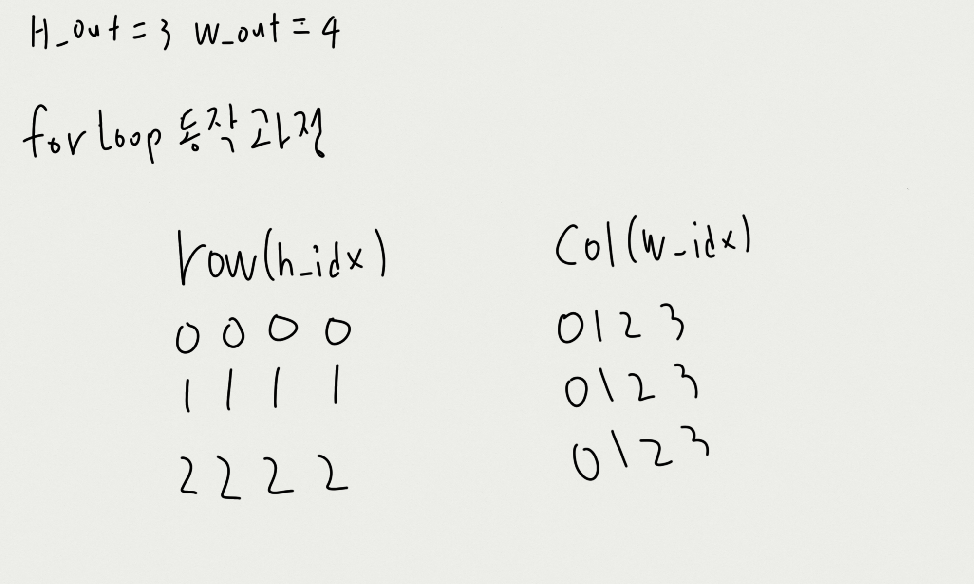
for문 전체가 동작하는 동안 row, col은 위 그림과 같은 모습일 것이다.
일단은 저 친구들을 일반화해서 만들어 보면
import numpy as np
from numpy.random import randint

H_in, W_in = 5, 6

F = 3
X = randint(0, 10, (H_in, W_in))

W = randint(0, 10, (F, F))
B = randint(0, 10, ())
H_out, W_out = H_in - F + 1, W_in - F + 1

print(H_out, W_out) # 3 4

Z = np.empty(shape=(H_out, W_out))

# for row_idx in range(H_out):
#     for col_idx in range(W_out):
#         print(f"({row_idx}, {col_idx})", end="\t")
#     print()
# (0, 0)  (0, 1)  (0, 2)  (0, 3)
# (1, 0)  (1, 1)  (1, 2)  (1, 3)
# (2, 0)  (2, 1)  (2, 2)  (2, 3)

print(np.arange(H_out))
# [0 1 2]

print(np.repeat(np.arange(H_out), W_out))
# [0 0 0 0 1 1 1 1 2 2 2 2]

print(np.arange(H_out).reshape(-1, 1))
# [[0]
# [1]
# [2]]

print(np.repeat(np.arange(H_out).reshape(-1, 1), W_out, axis=-1))
# [[0 0 0 0]
#  [1 1 1 1]
#  [2 2 2 2]]

# Make row index
row_idx = np.arange(H_out)
row_idx = row_idx.reshape(-1,1)
row_idx = np.repeat(row_idx, W_out, axis=-1)
print(row_idx)
# [[0 0 0 0]
#  [1 1 1 1]
#  [2 2 2 2]]

print(np.arange(W_out))
# [0 1 2 3]
print(np.tile(np.arange(W_out), H_out))
# [0 1 2 3 0 1 2 3 0 1 2 3]
print(np.tile(np.arange(W_out), H_out).reshape(H_out, W_out))
# [[0 1 2 3]
#  [0 1 2 3]
#  [0 1 2 3]]

# Make col index - method 1
col_idx = np.arange(W_out)
col_idx = np.tile(col_idx, H_out)
col_idx = col_idx.reshape(H_out,W_out)
print(col_idx)
# [[0 1 2 3]
#  [0 1 2 3]
#  [0 1 2 3]]


# Make col index - method 2
col_idx = np.arange(W_out)
col_idx = np.tile(col_idx, [H_out, 1])
print(col_idx)
# [[0 1 2 3]
#  [0 1 2 3]
#  [0 1 2 3]]
만들어지는 과정을 단계별로 천천히 밟아봤다.
이 과정을 밟으면, 우리가 그림을 통해 살펴봤던 for문 동작 과정 중의 row, col index를 얻었다.
그런데, 여기서 끝이 아니다.
우리는 이 index들을 가지고 "window"를 추출해야 한다. 연산은 "window"를 기준으로 수행하니까
4.3 for loop의 동작 과정 with window
우리가 위에서 찾은 row, col index를 가지고 window를 만들어 보면, 아래 그림처럼 만들어질 것이다.

위 그림을 window를 중심으로 다시 그려보면

느낌과 이미지를 알기 위해서 그림을 그렸는데, 이 matrix를 indexing을 통해 어떻게 가져와야 할까 머리가 아프다.
그리고 하나의 발상 "벡터화"
4.4 Vectorization(벡터화)

그래. 벡터화를 해보자
(row_idx, col_idx)가 (0, 0) 일 경우의 filter를 벡터화해보자

(0, 0)의 window는 위와 같이 나올 것이다.
그러면 전체 window를 벡터화해서 쭉 늘려보자
import numpy as np
from numpy.random import randint

H_in, W_in = 5, 6

F = 3
X = randint(0, 10, (H_in, W_in))

W = randint(0, 10, (F, F))
B = randint(0, 10, ())
H_out, W_out = H_in - F + 1, W_in - F + 1

print(H_out, W_out) # 3 4

Z = np.empty(shape=(H_out, W_out))

# Make row index
row_idx = np.arange(H_out)
print(row_idx)
# [0 1 2]

row_idx = row_idx.reshape(-1,1)
print(row_idx)
# [[0]
#  [1]
#  [2]]

row_idx = np.repeat(row_idx, W_out, axis=-1)
print(row_idx)
# [[0 0 0 0]
#  [1 1 1 1]
#  [2 2 2 2]]

row_idx = row_idx.reshape(-1, 1)
print(row_idx)
# [[0]
#  [0]
#  [0]
#  [0]
#  [1]
#  [1]
#  [1]
#  [1]
#  [2]
#  [2]
#  [2]
#  [2]]

window_row = np.repeat(np.arange(F), F).reshape(1, -1)
print(window_row)
# [[0 0 0 1 1 1 2 2 2]]

row_idx = row_idx + window_row
print(row_idx)
# [[0 0 0 1 1 1 2 2 2]
#  [0 0 0 1 1 1 2 2 2]
#  [0 0 0 1 1 1 2 2 2]
#  [0 0 0 1 1 1 2 2 2]
#  [1 1 1 2 2 2 3 3 3]
#  [1 1 1 2 2 2 3 3 3]
#  [1 1 1 2 2 2 3 3 3]
#  [1 1 1 2 2 2 3 3 3]
#  [2 2 2 3 3 3 4 4 4]
#  [2 2 2 3 3 3 4 4 4]
#  [2 2 2 3 3 3 4 4 4]
#  [2 2 2 3 3 3 4 4 4]]

print(row_idx.shape)
# (12, 9)

# Make col index - method 2
col_idx = np.arange(W_out)
print(col_idx)
# [0 1 2 3]

col_idx = np.tile(col_idx, [H_out, 1])
print(col_idx)
# [[0 1 2 3]
#  [0 1 2 3]
#  [0 1 2 3]]

col_idx = col_idx.reshape(-1, 1)
print(col_idx)
# [[0]
#  [1]
#  [2]
#  [3]
#  [0]
#  [1]
#  [2]
#  [3]
#  [0]
#  [1]
#  [2]
#  [3]]

window_col = np.tile(np.arange(F), F).reshape(1, -1)
print(window_col)
# [[0 1 2 0 1 2 0 1 2]]

col_idx = col_idx + window_col
print(col_idx)
# [[0 1 2 0 1 2 0 1 2]
#  [1 2 3 1 2 3 1 2 3]
#  [2 3 4 2 3 4 2 3 4]
#  [3 4 5 3 4 5 3 4 5]
#  [0 1 2 0 1 2 0 1 2]
#  [1 2 3 1 2 3 1 2 3]
#  [2 3 4 2 3 4 2 3 4]
#  [3 4 5 3 4 5 3 4 5]
#  [0 1 2 0 1 2 0 1 2]
#  [1 2 3 1 2 3 1 2 3]
#  [2 3 4 2 3 4 2 3 4]
#  [3 4 5 3 4 5 3 4 5]]

print(col_idx.shape)
# (12, 9)
정신없는데 중요한 부분만 봐보자
row_idx = row_idx + window_row
print(row_idx)
# [[0 0 0 1 1 1 2 2 2]
#  [0 0 0 1 1 1 2 2 2]
#  [0 0 0 1 1 1 2 2 2]
#  [0 0 0 1 1 1 2 2 2]
#  [1 1 1 2 2 2 3 3 3]
#  [1 1 1 2 2 2 3 3 3]
#  [1 1 1 2 2 2 3 3 3]
#  [1 1 1 2 2 2 3 3 3]
#  [2 2 2 3 3 3 4 4 4]
#  [2 2 2 3 3 3 4 4 4]
#  [2 2 2 3 3 3 4 4 4]
#  [2 2 2 3 3 3 4 4 4]]

print(row_idx.shape)
# (12, 9)

col_idx = col_idx + window_col
print(col_idx)
# [[0 1 2 0 1 2 0 1 2]
#  [1 2 3 1 2 3 1 2 3]
#  [2 3 4 2 3 4 2 3 4]
#  [3 4 5 3 4 5 3 4 5]
#  [0 1 2 0 1 2 0 1 2]
#  [1 2 3 1 2 3 1 2 3]
#  [2 3 4 2 3 4 2 3 4]
#  [3 4 5 3 4 5 3 4 5]
#  [0 1 2 0 1 2 0 1 2]
#  [1 2 3 1 2 3 1 2 3]
#  [2 3 4 2 3 4 2 3 4]
#  [3 4 5 3 4 5 3 4 5]]

print(col_idx.shape)
# (12, 9)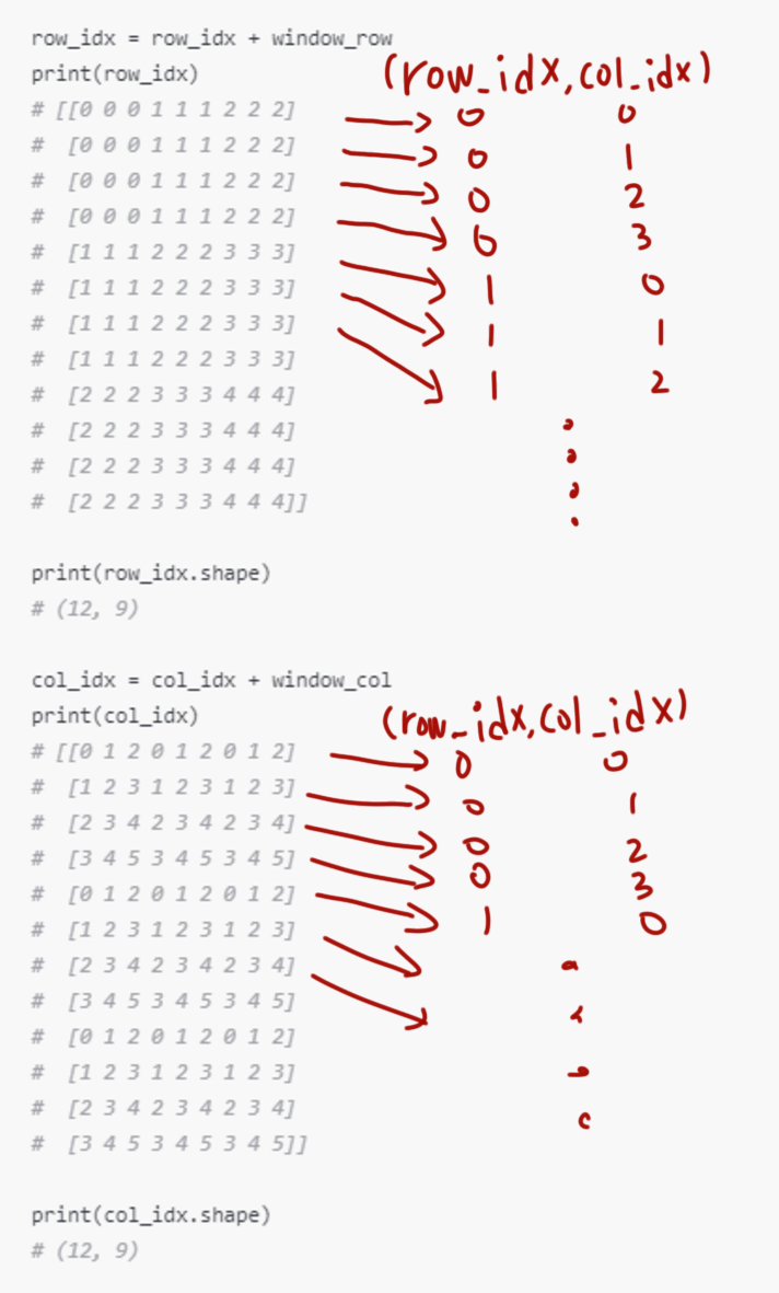
위와 같이 row_idx, col_idx를 구하게 됐을 때,
만약 X[row_idx[0], col_idx[0]]의 값을 바라본다면
X[row_idx[0], col_idx[0]] = for문 row_idx: 0, col_idx: 0일 때 window, 그 window의 Vectorization이다.
그러면, 벡터화한 이 데이터는 어떻게 연산이 될까?
당연히 벡터 간의 연산 Dot Product다
import numpy as np
from numpy.random import randint

H_in, W_in = 5, 6

F = 3
X = randint(0, 10, (H_in, W_in))

W = randint(0, 10, (F, F))
B = randint(0, 10, ())
H_out, W_out = H_in - F + 1, W_in - F + 1

print(H_out, W_out) # 3 4

Z = np.empty(shape=(H_out, W_out))

# Make window row index
row_idx = np.arange(H_out)
row_idx = row_idx.reshape(-1,1)
row_idx = np.repeat(row_idx, W_out, axis=-1)
row_idx = row_idx.reshape(-1, 1)
window_row = np.repeat(np.arange(F), F).reshape(1, -1)
row_idx = row_idx + window_row
print(row_idx.shape)
# (12, 9)

# Make window col index
col_idx = np.arange(W_out)
col_idx = np.tile(col_idx, [H_out, 1])
col_idx = col_idx.reshape(-1, 1)
window_col = np.tile(np.arange(F), F).reshape(1, -1)
col_idx = col_idx + window_col
print(col_idx.shape)
# (12, 9)

# window의 index를 실제 window 값
windows = X[row_idx, col_idx]
print(windows.shape)    # (12, 9)
W = W.reshape(-1, 1)
print(W.shape)  # (9, 1)

Z = windows @ W + B
print(Z.shape)  # (12, 1)

Z = Z.reshape(H_out, W_out)
print(Z.shape)  # (3, 4)
맨 밑 연산과정을 다시 살펴보자
windows = X[row_idx, col_idx]
print(windows.shape)    # (12, 9)
W = W.reshape(-1, 1)
print(W.shape)  # (9, 1)

Z = windows @ W + B
print(Z.shape)  # (12, 1)

Z = Z.reshape(H_out, W_out)
print(Z.shape)  # (3, 4)
우리가 알고 있던 Dot Product 연산이 진행돼서, 다시 reshape 해서 우리가 원하는 결과를 얻어냈다.
복잡한 과정을 겪어 결과를 얻었는데, 이 결과가 얼마나 효율적인지, 시간을 절약하는지 확인해보자
기존 for문 연산과 벡터화 연산의 걸리는 차이를 확인해보자
import numpy as np
import matplotlib.pyplot as plt
from time import time

img = plt.imread('./고먐미_1.jpg')
img_gray = np.mean(img, axis=-1).astype(np.int32)

H_in, W_in = img_gray.shape
print(H_in, W_in)
# 1125 1125

F = 3
X = img_gray

W = np.full(fill_value=1/(F*F), shape=(F, F))

H_out, W_out = H_in - F + 1, W_in - F + 1
print(H_out, W_out)
# 1123 1123

Z_wo = np.empty(shape=(H_out, W_out))

# method 1
start_wo_vec = time()
for row_idx in range(H_out):
    for col_idx in range(W_out):
        window = X[row_idx : row_idx + F,
                    col_idx : col_idx + F]
        z = np.sum(window * W)
        Z_wo[row_idx, col_idx] = z
end_wo_vec = time()
elapsed_time_wo_vec = end_wo_vec - start_wo_vec
print(elapsed_time_wo_vec * 1000)
# 7402.255296707153

# method 2
row_idx = np.arange(H_out)
row_idx = row_idx.reshape(-1,1)
row_idx = np.repeat(row_idx, W_out, axis=-1)
row_idx = row_idx.reshape(-1, 1)
window_row = np.repeat(np.arange(F), F).reshape(1, -1)
row_idx = row_idx + window_row

col_idx = np.arange(W_out)
col_idx = np.tile(col_idx, [H_out, 1])
col_idx = col_idx.reshape(-1, 1)
window_col = np.tile(np.arange(F), F).reshape(1, -1)
col_idx = col_idx + window_col

start_w_vec = time()
windows = X[row_idx, col_idx]
W = W.reshape(-1, 1)

Z = windows @ W
Z_w = Z.reshape(H_out, W_out)
end_w_vec = time()

elapsed_time_w_vec = end_w_vec - start_w_vec
print(elapsed_time_w_vec * 1000)
# 138.01813125610352
print(f"걸린 시간 몇배 ? {elapsed_time_wo_vec / elapsed_time_w_vec}")
# 걸린 시간 몇배 ? 53.63248458256318

fig, ax = plt.subplots(1, 3, figsize=(10, 20))
ax[0].imshow(img_gray, cmap="gray")
ax[1].imshow(Z_wo, cmap="gray")
ax[2].imshow(Z_w, cmap="gray")

plt.show()
3x3 filter의 경우에는 53배의 차이가 난다. 어마어마한 차이다.
"나만 잘한다면" 수십 배의 시간 절약을 할 수 있겠다.
그런데 for문을 없애는 벡터화에도 단점은 있다.
1. 메모리를 많이 잡아먹는다. (30x30 filter는 메모리 부족으로 실행 불가)
2. 벡터가 길어지면, 결과가 비슷해진다. (15x15 filter부터는 1, 2배 정도로 거의 비슷해지는 수준)
* 참조
- https://ko.wikipedia.org/wiki/%ED%95%A9%EC%84%B1%EA%B3%B1_%EC%8B%A0%EA%B2%BD%EB%A7%9D
합성곱 신경망 - 위키백과, 우리 모두의 백과사전
ko.wikipedia.org


댓글